2 Introduction to the course
“There is grandeur in this view of life, with its several powers, having been originally breathed into a few forms or into one; and that, whilst this planet has gone cycling on according to the fixed law of gravity, from so simple a beginning endless forms most beautiful and most wonderful have been, and are being, evolved.”
The above quotation is one of the most iconic ones in biology. It beautifully concludes The Origin of Species by Charles R. Darwin, emphasizing the diversity of forms that we can find in nature, and how natural selection can shape these forms. Indeed, even in a simple walk through our neighborhood we can find hundreds of organisms, from plants to animals, with varying forms. From this observation, a natural question is then, how all these forms came to be?
To answer this question, we need to address two main problems. First, we need to assess the set of processes that act as a source of heritable variation on traits. Then, we need to understand how a second set of processes act upon the available heritable variation and shape traits. Our course focuses on this second problem. Specifically, we will study the theory and the mathematical foundations behind one of the main processes that can act upon heritable variation in populations: natural selection.
Throughout the first block, we will derive from first principles and gain some intuition about the main equations that predict how natural selection should drive evolution. In the second block, we will then use these equations to study ecological interactions as a source of reciprocal selective pressures that drive the coevolution between species.
2.1 The fundamental concepts of evolution by natural selection
First things first, we need a definition of evolution so that we can start from there. Following Futuyma (2005), evolution can be defined as a “change in the properties of groups of organisms over the course of generations”. Note that the properties in this definition of evolution “…embraces everything from slight changes in the proportions of different forms of a gene within a population to the alterations that led from the earliest organism to dinosaurs, bees, oaks, and humans” (Futuyma 2005). Throughout the course we will focus on how natural selection can drive the evolution of properties that can be measured as discrete or continuous traits in a population. Two biological examples of discrete and continuous traits would be the frequency of alleles that determine discrete floral morphs, or the length of floral tubes in population of plants, respectively. We will also focus on how these traits change within populations, or microevolutionary changes, in contrast with changes that could occur above the level of species, or macroevolutionary changes (Turner et al. 2009).
With this definition in hand, our first question is then how natural selection can drive changes in discrete or continuous traits in populations from one generation to the other? Before attempting to answer the question, we also need to define natural selection. Definitions are important because they allow us to build our models from fundamental propositions and assumptions that we know are true, or, the so called first principles. We can define natural selection as the differential survival and reproduction of individuals due to differences in heritable traits (Rice 2004). From this definition we can identify the three fundamental propositions that allow natural selection to operate:
Traits need to vary between individuals in a population.
These traits need to be heritable.
Individuals with different traits need to differ in how much they contribute with reproduction to the next generation.
In evolutionary biology the word fitness is used to convey the reproductive contribution of an individual to the next generation (Rice 2004), and this is the definition of fitness that we will use throughout this course. Now that we have defined the scope of our problem (microevolution of discrete and continuous traits) and the first principles underlying our process of interest (the three propositions of natural selection), we can start to mathematically describe the problem.
2.2 Natural selection and the evolution of allele frequencies within populations
2.2.1 Building our first equation
Natural populations are complex, and it would be impossible to incorporate all the details that we can find when we mathematically describe a problem. Not only it would be impossible, but it would severely hinder our ability to understand and disentangle how our process of interest operates. Thus, our first step is to make some simplifying assumptions about these populations. Understanding what simplifying assumptions are reasonable is a complex topic and to learn more about this problem I highly recommend starting with the classic paper by Richard Levins, The strategy of model building in population biology. The short answer is that the choice of simplifying assumptions depends on your problem of interest and the questions that you are trying to answer.
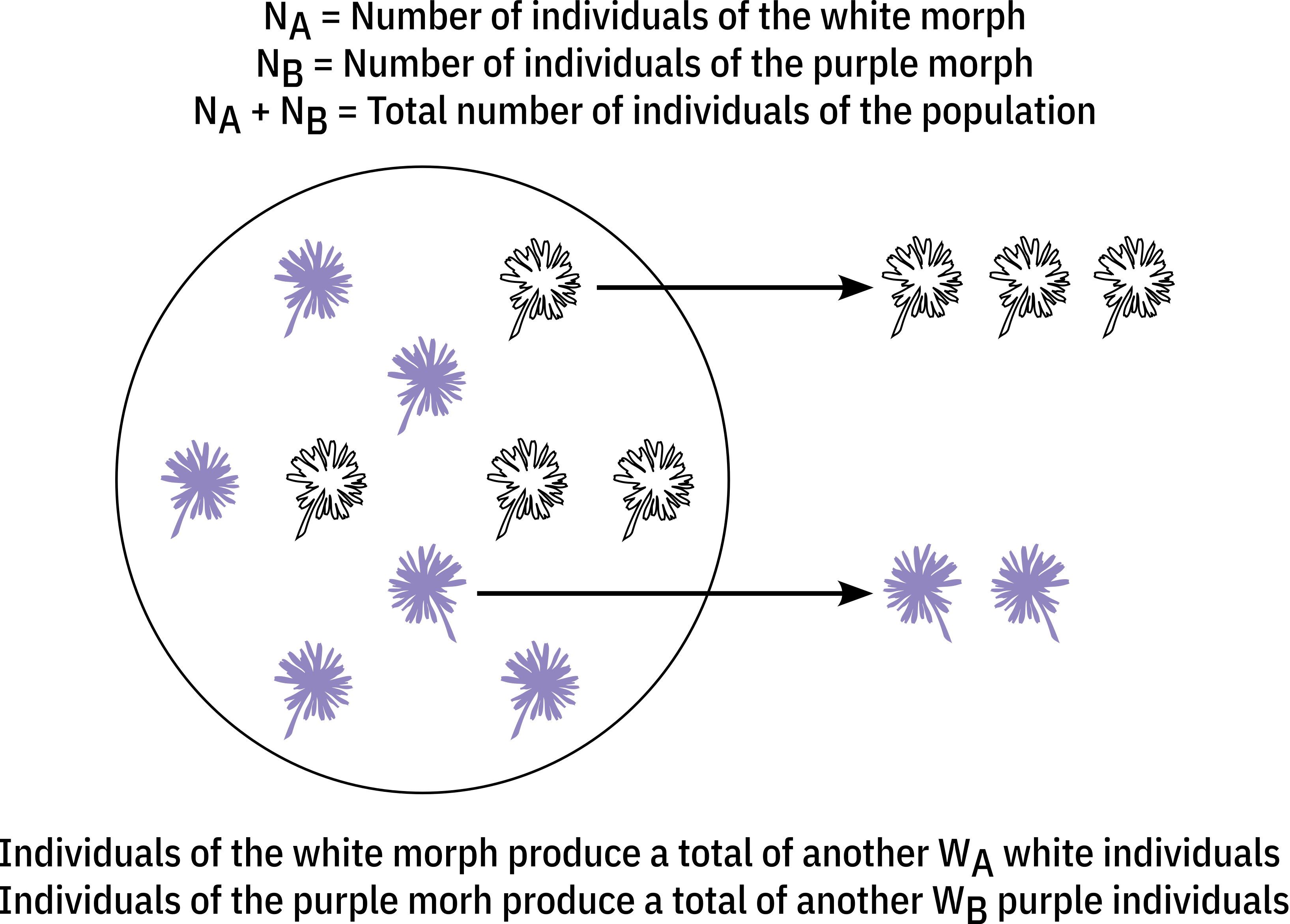
Here, we are concerned about how populations evolve by means of natural selection. So, our first simplifying assumption is that the only mechanism of evolutionary change within a population is natural selection and that generations are non-overlapping. Our next step is to incorporate the fundamental propositions through which natural selection operates. The first one is that individuals vary in their traits. For these traits, we will assume the simplest case, in which a population contains individuals with only two discrete morphs/traits, for instance, plant individuals that produce only white flowers or purple flowers. From the second proposition, these traits need to be heritable. So, we will also assume that individuals are haploid, that two alleles, \(A\) and \(B\), determine the two morphs (e.g. the white and purple morphs), and that these alleles are inherited by the offspring of individuals. Finally, each of the \(N_A\) or \(N_B\) individuals carrying the \(A\) or \(B\) alleles contributes to the next generation with an amount of \(W_A\) and \(W_B\) of individuals that inherit the \(A\) and \(B\) alleles, respectively. Thus, \(W_A\) and \(W_B\) represent the fitness of these individuals. Figure 1 below illustrates this scenario using the example of plant individuals displaying white or purple flowers.
\(\\\)
Under the above assumptions, in the next generation the total number of individuals carrying the allele \(A\) in the population will depend on how much each individual contribute with offspring to the next generation. Mathematically, this is equivalent to multiply the current number of individuals carrying the allele \(A\), with their fitness, as follows:
\[N_{A}^{(t+1)}=N_{A}^{(t)}W_{A}^{(t)}\]
where the superscripts \((t)\) and \((t+1)\) denotes the current and the next generation, respectively. Similarly, the following equation describes the number of individuals carrying the \(B\) allele in the next generation: \[N_{B}^{(t+1)}=N_{B}^{(t)}W_{B}^{(t)}\] However, we are interested in how the frequencies of these alleles change, not the absolute number of individuals. Since there are only two alleles in the population, if we find the frequency - \(p\) - of allele \(A\), then the frequency of \(B\) is equal to \((1-p)\). The frequency of \(A\) in the next generation is equal to the number of individuals carrying \(A\), divided by total number of individuals in the next generation, \(\frac{N_{A}^{(t+1)}}{N^{(t+1)}}\). We already know what \(N_{A}^{(t+1)}\) is, so our next step is to find what will be the total number of individuals in the next generation, \(N^{(t+1)}\). From the two equations above, we know that the total population size at the next generation is equal to:
\[N^{(t+1)}=N_{A}^{(t)}W_{A}^{(t)}+N_{B}^{(t)}W_{B}^{(t)}\]
We also know that at the current generation, the number of individuals carrying the allele \(A\), \(N_{A}^{(t)}\), is equal to the frequency of \(A\), multiplied by the total number of individuals in the population, that is \(N_{A}^{(t)}=p^{(t)}N^{(t)}\). In a similar way, \(N_{B}^{(t)}=(1-p^{(t)})N^{(t)}\). If we plug in these equivalences in the equation above, we get to the following one:
\[ \begin{aligned} N^{(t+1)}&=N_{A}^{(t)}W_{A}^{(t)}+N_{B}^{(t)}W_{B}^{(t)} \\ N^{(t+1)}&=p^{(t)}N^{(t)}W_{A}^{(t)}+(1-p^{(t)})N^{(t)}W_{B}^{(t)} \end{aligned} \]
Further putting the \(N^{(t)}\) that appears at the right-hand side in evidence leads to:
\[ \begin{aligned} N^{(t+1)}&=p^{(t)}N^{(t)}W_{A}^{(t)}+(1-p^{(t)})N^{(t)}W_{B}^{(t)} \\ N^{(t+1)}&=N^{(t)}\left[p^{(t)}W_{A}^{(t)}+(1-p^{(t)})W_{B}^{(t)} \right] \\ N^{(t+1)}&=N^{(t)}\overline{W}^{(t)} \end{aligned} \] where \(\overline{W}^{(t)}=p^{(t)}W_{A}^{(t)}+(1-p^{(t)})W_{B}^{(t)}\) is the average fitness of the population.
\[\begin{aligned} \frac{N_{A}^{(t+1)}}{N^{(t+1)}}&=\frac{N_{A}^{(t)}W_{A}^{(t)}}{N^{(t)}\overline{W}^{(t)}} \\ p^{(t+1)}&=\frac{p^{(t)}W_{A}^{(t)}}{\overline{W}^{(t)}} \end{aligned}\]
Now, lets try to understand what the equation above is telling us: at the next generation, the frequency of the allele \(A\) in the population will depend on the current frequency of \(A\), multiplied by the fraction \(\frac{W_{A}^{(t)}}{\overline{W}^{(t)}}\). This fraction represents the fitness of \(A\) relative to the average fitness in the population. On the one hand, if the fitness of \(A\) is larger than the average of the population, the fraction is higher than 1, and the frequency of \(A\) will increase in the next generation. On the other hand, when \(W_{A}^{(t)} < \overline{W}^{(t)}\), the fraction will be smaller than 1 and the frequency of \(A\) will decrease. What the equation is describing makes complete sense. If individuals of \(A\) reproduce more than the average, then, the frequency of \(A\) increases. This is exactly the way that we expect natural selection to operate, but now, we are able to quantify this expected outcome.
2.2.2 Wright’s equation for the adaptive landscape of alleles
We can gain further insight about how selection drive the frequencies of alleles if we come up with an expression for the change in the frequency over generations, instead of just the frequency at the next generation. Mathematically, this is described by the difference \(p^{(t+1)} - p^{(t)}\), or \(\Delta p\) . Plugging in the expression for \(p^{(t+1)}\) that we just derived leads to the following equation:
\[\begin{aligned} \Delta p&=p^{(t+1)} - p^{(t)} \\ \Delta p&=\frac{p^{(t)}W_{A}^{(t)}}{\overline{W}^{(t)}} - p^{(t)} \\ \Delta p&=\frac{p^{(t)}W_{A}^{(t)}}{\overline{W}^{(t)}} - \frac{p^{(t)}\overline{W}^{(t)}}{\overline{W}^{(t)}} \\ \Delta p&=p^{(t)}\frac{\left(W_{A}^{(t)}-\overline{W}^{(t)}\right)}{\overline{W}^{(t)}} \end{aligned}\]
Substituting \(\overline{W}^{(t)}\) in the numerator with \(p^{(t)}W_{A}^{(t)}+(1-p^{(t)})W_{B}^{(t)}\) leads to:
\[\begin{aligned} \Delta p&=p^{(t)}\frac{\left[W_{A}^{(t)}-p^{(t)}W_{A}^{(t)}-(1-p^{(t)})W_{B}^{(t)}\right]}{\overline{W}^{(t)}} \\ \Delta p&=p^{(t)}\frac{\left[(1-p^{(t)})W_{A}^{(t)}-(1-p^{(t)})W_{B}^{(t)}\right]}{\overline{W}^{(t)}} \\ \Delta p&=p^{(t)}(1-p^{(t)})\frac{\left(W_{A}^{(t)}-W_{B}^{(t)}\right)}{\overline{W}^{(t)}} \end{aligned}\]
This equation show that the change in the frequency of the \(A\) allele depends on two components. First, it depends on \(p^{(t)}(1-p^{(t)})\). This term is the product of the frequencies of \(A\) and \(B\), which, from probability theory, represents the variance in frequencies. From this interpretation, the term \(p^{(t)}(1-p^{(t)})\) is the amount of genetic variance within the population. Second, the change in frequency also depends on the term \(\frac{\left(W_{A}-W_{B}^{(t)}\right)}{\overline{W}^{(t)}}\), representing the difference in fitness between individuals carrying the \(A\) or \(B\) alleles. When \(W_{A}>W_{B}\), this term is positive and it is negative when \(W_{A}<W_{B}\). Therefore, the equation shows that selection drives evolutionary changes depending on the amount of the available genetic variance within the population and differences in fitness. On the one hand genetic variance scales the amount of evolutionary change that can occur, such that if there is no genetic variance, i.e., \(p\neq 1\) and \(p\neq 0\), no change occurs. On the other hand, differences in fitness control the direction of the evolutionary changes. Since the variance is always a positive number, when \(W_{A}>W_{B}\), \(\Delta p\) is also positive and the frequency of \(p\) increases. In contrast, when \(W_{A}<W_{B}\), \(\Delta p\) will be negative and the frequency of \(p\) decreases. If there are no differences in fitness, or \(W_{A} = W_{B}\), there is no evolutionary change. Once more, this behavior makes complete sense from what we would expect from evolution by natural selection.
The equation above for the change in allele frequencies was the one derived by Sewall Wright in 1937 in the classic paper The distribution of gene frequencies in populations. The key idea of the paper was identifying that the term \(\left(W_{A}^{(t)}-W_{B}^{(t)}\right)\) corresponds to the derivative of the average fitness of the population, relative to the frequency of allele \(p\), as follows:
\[\begin{aligned} \frac{\partial \overline{W}^{(t)}}{\partial p} &= \frac{\partial}{\partial p^{(t)}}p^{(t)}W_{A}^{(t)} + \frac{\partial}{\partial p^{(t)}}(1-p^{(t)})W_{B}^{(t)} \\ \frac{\partial \overline{W}^{(t)}}{\partial p^{(t)}} &= W_{A}^{(t)} - W_{B}^{(t)} \end{aligned}\]
This result holds whenever the fitness of alleles does not depend on their frequencies, or, in other words, when fitness is frequency independent. The result above allow us to rewrite the equation for the change in allele frequencies as follows:
\[ \Delta p=p^{(t)}(1-p^{(t)})\frac{\partial ln\overline{W}^{(t)}}{\partial p^{(t)}} \] where the ln term in \(\frac{\partial ln\overline{W}^{(t)}}{\partial p^{(t)}}\) comes from the calculus rule that \(\frac{1}{x}\frac{d}{dx} = \frac{dlnx}{dx}\).
Rewriting the equation in terms of this derivative is key to understand the concept of how natural selection drive adaptations in populations. A derivative represents the slope of a curve at a point. In turn, the average fitness of a population represents its growth rate. Thus, we can think about the derivative of the average fitness relative to the frequency of an allele as a population “climbing” a slope that is defined by the growth rate of the population. Visually this can be represented with the relationship between the average fitness of the population and the frequency of a given allele, as the figure below shows:
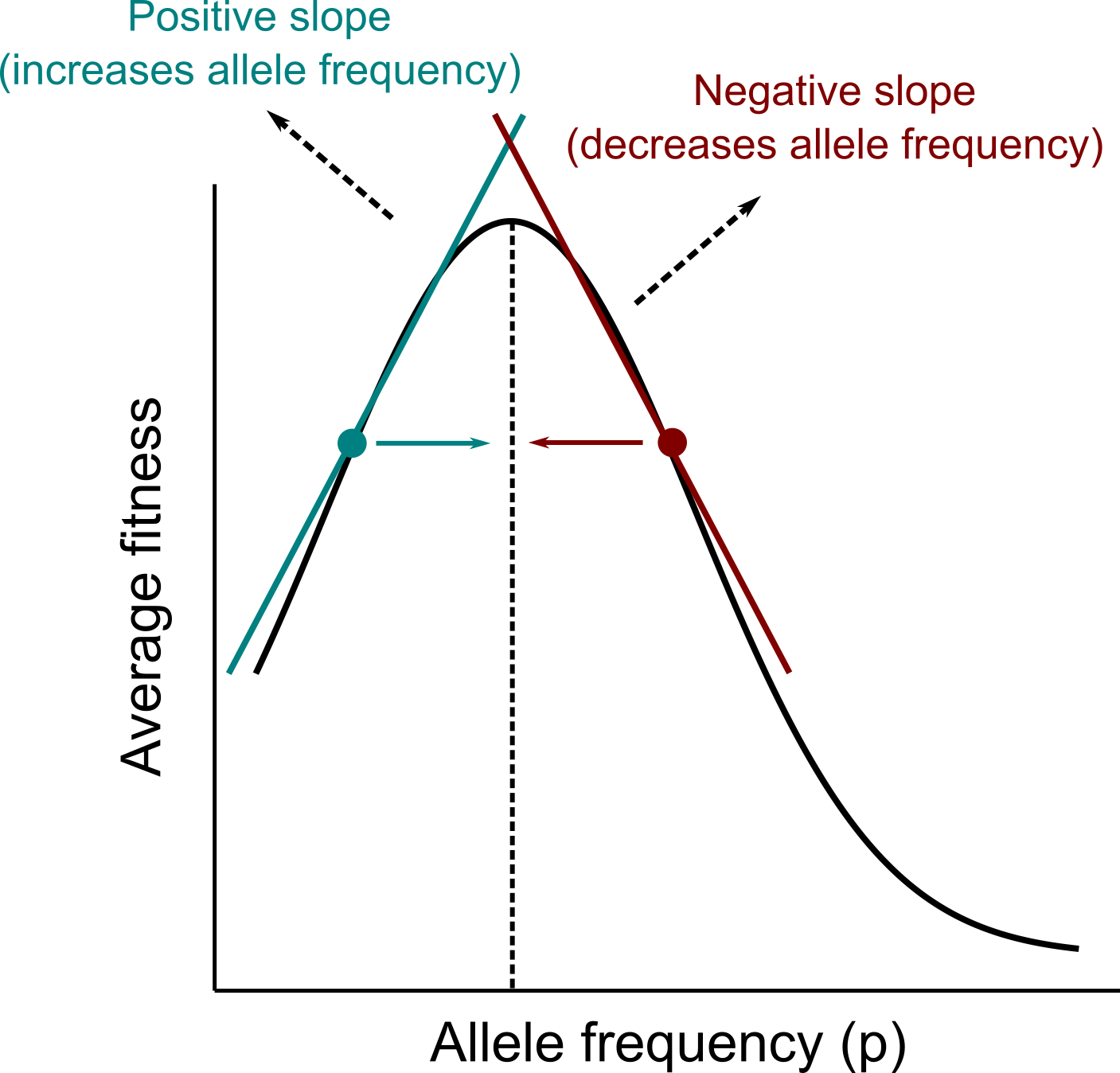
\(\\\)
The figure above illustrates the concept introduced by Wright (1937) of an adaptive landscape. In evolutionary biology, the adaptive landscape depicts the relationship between the average fitness of a population and the values of traits, which, in our example, are the frequencies of alleles. From the figure and the interpretation of the derivative outlined above, we can see the natural selection will drive the evolution of allele frequencies in the direction that increases the average fitness of the population. This provides a mathematical formulation and proof of the intuitive concept of how natural selection favors adaptations in populations. This relationship always holds whenever fitness is frequency-independent, but not when fitness is frequency-dependent as we will see next in the exercise session.
Going back to our initial question: how natural selection can drive changes in discrete or continuous traits in populations from one generation to the other? Using Wright’s equation we now can partially answer this question. For discrete traits, for instance, alleles, we learned that selection will favor the evolution of an increased frequency of alleles that maximize the average fitness of the population, leading to adaptations. The rate at which the population evolves will depend on the available genetic variation in the population, as well as how large are the differences in fitness between individuals carrying different alleles.
2.2.3 References
Darwin, Charles Robert. 1861. On the Origin of Species by Means of Natural Selection, or the Preservation of Favoured Races in the Struggle for Life. 3d edition. London: John Murray.
Futuyma, Douglas. 2005. Evolution. Sunderland, MA: Sinauer Associates.
Levins, R. 1966. The strategy of model building in population biology. American Scientist 54 (4): 421–31.
Rice, Sean H. 2004. Evolutionary Theory: Mathematical and Conceptual Foundations. New York, NY: Oxford University Press.
Turner, Derek and Joyce C. Havstad. 2019. Philosophy of Macroevolution. The Stanford Encyclopedia of Philosophy (Summer 2019 Edition), Edward N. Zalta (ed.). Available in: https://plato.stanford.edu/archives/sum2019/entries/macroevolution.
Wright, S. 1937. The distribution of gene frequencies in populations. Proceedings of the National Academy of Sciences of the United States of America 23 (6): 307–20.